Making Moirai Recursive
to improve long horizon time series forecasting
TL;DR
Moirai 2 is a time-series foundation model released by Salesforce. To make distributional forecasts, it predicts quantiles for every step in a horizon (64 by default). For longer horizons, the model uses a procedure similar to beam search to autoregress. We show that training the model instead to recurse a latent state yields better distributional long-range forecasts. The approach increases training cost and cannot use conventional KV caching, but simplifies decoding.
Moirai 2
After reading the first foundational time-series papers like Chronos a few years ago, I was curious to see how approaches had evolved. Moirai 2 stood out for its simplicity:
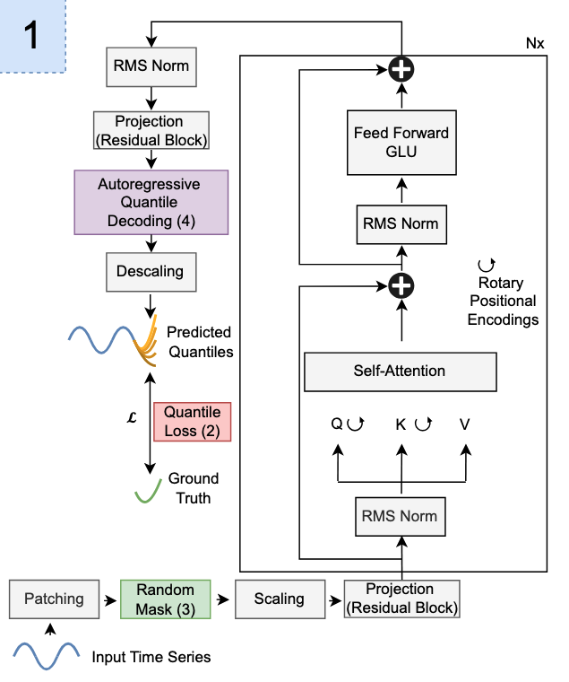
Univariate series are split into non-overlapping chunks (patches) of size 16, scaled, and embedded with a residual block before entering a standard decoder-only transformer. Causal attention operates at the patch level and the transformer output is decoded with another residual block. The network outputs predictions for 9 quantiles (0.1, 0.2, …, 0.9) for each of 64 future time steps (4 patches of size 16). Training using the quantile (pinball) loss at each of the 9 levels teaches the model to estimate probabilistic forecasts.
A few papers like Chronos-Bolt and Moirai 2 have opted to directly decode a chunk of future observations instead of generating one at a time to combat error accumulation from autoregression. However, models still have to autoregress when horizons are longer than they were directly trained to predict.
Autoregressing is not as simple because the model outputs predictions for all nine quantiles, but expects a one-dimensional input. So, what value should models append to the context to predict the next chunk? Moirai 2 proposes to expand the context with each of the predicted nine quantiles independently to obtain (9 x 9 = 81) “candidate” predictions for the next chunk. To get the final predictions they collapse the candidates from 81 to 9 by calculating the empirical quantiles at each timestep. Repeat until the forecast is the desired length.
While their ablations show their “expand-collapse” decoding improves performance over taking the median, I thought it could maybe be improved.
Recursing latents instead of values
The transformer input and output shapes already match. What if instead of recursing the quantiles, we treat the transformer outputs as RNN-like hidden or latent states and roll those?
We could simply feed the transformer output back into it at test-time to predict the next chunk. But without modifying training, the transformer won’t have seen its own outputs as inputs or know to map them 1.
So, during training we recurse the latent and supervise the max_unrolls 64-observation chunks. The longest horizons in the main benchmark the authors report (GIFT-Eval) are around 900 observations, meaning that if we want those in-distribution, we should aim for about 15 or so unrolls.
Of course, backpropagating through that many forwards is impossible without absurd hardware, and likely unnecessary. We supervise every rollout but detach the latent every bptt_window unrolls.
Predicting both short and long horizons are not equally difficult or important, so we weighted chunks’ losses differently:
- In a first approach we simply geometrically decayed weights: \(w_k = \alpha^k\).
- To try to eliminate the decay hyperparameter (or replace with a more robust one), we kept track of an EMA of each chunk’s loss (\(e_k\)) and weight inversely proportional to it: \(w_k \propto 1 / (e_k + \epsilon)\).
There was also a question of what to recurse and if we should add depth embeddings. At first, we had empirically landed on:
inp = latent + stop_grad(emb) + depth_emb(k) + feedback(latent)
latent = transformer(inp)
where emb is the series’ original embedding, latent the previous rollout’s transformer output, depth_emb a fixed sinusoidal embedding, and feedback a simple zero-initialized linear layer.
Results
Since the Moirai paper didn’t provide the exact data mix or their internal CloudOps telemetry data, we try a few different mixes for the public sets and arrive at 48/20/20/12% for GIFT-Pretrain, GIFT-TrainTest, Chronos-Mixup, and Kernel-Synth respectively. Models train for 100k steps and we try to replicate Moirai’s setup as closely as possible but omit sequence packing for simplicity and increase patch size (16 -> 32) since we measured equivalent performance at higher throughput.
The GIFT-Eval Benchmark has 97 dataset-horizon combinations and reports the geometric mean of seasonal-naive-normalized CRPS and MASE across tasks (lower is better). We report CRPS by forecast length and also include calibration metrics which are averaged arithmetically.
Our best recursive model trains with 12 unrolls (with a reach of 768), a BPTT window of 2, the recurrence described above and geometric decay on the loss with \(\alpha = 0.7\). The direct-depth control predicts each future block independently from the original context and its depth encoding, without carrying a latent state. Results with three seeds:
| Config | CRPS | Short | Medium | Long | MASE | Cal. | Long 80% cov. |
|---|---|---|---|---|---|---|---|
| baseline | 0.5392 | 0.5556 | 0.5175 | 0.5193 | 0.7650 | 0.0718 | 0.5322 |
| recursive | 0.5399 | 0.5654 | 0.5147 | 0.5019 | 0.7748 | 0.0545 | 0.7458 |
| direct-depth | 0.5554 | 0.5773 | 0.5439 | 0.5124 | 0.8054 | 0.0552 | 0.7524 |
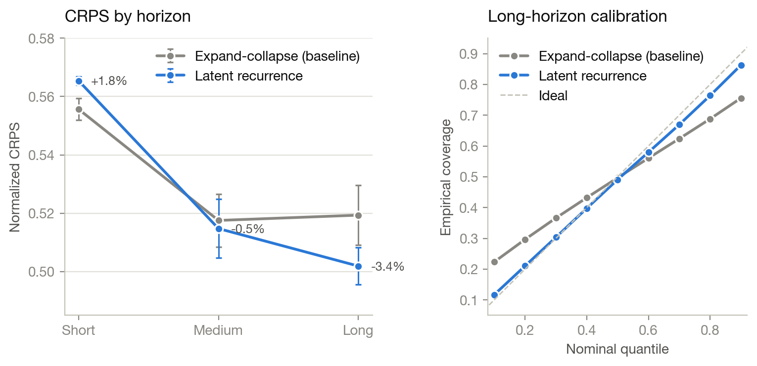
As you can see, the recursive model performs slightly worse for short horizons but improves for long ones. The overall CRPS is essentially tied because the benchmark contains 55 short settings but only 21 long ones. Calibration is what the recursive model improves on the most, with 24% lower error overall, and 44% lower error for long horizons. The right figure shows that expand-collapse decoding doesn’t do enough to preserve uncertainty since its predictions are too narrow.
The direct-depth control shows that long horizon supervision is not enough to match the recursive model’s performance. Note, however, that it does match its calibration.
While we could keep the baseline and recursive models and route between them for best performance, we attempted to address the tradeoff with a single model without much luck. As in the Moirai paper, increasing capacity gave diminishing returns and didn’t eliminate the tradeoff.
| Config | Params (M) | CRPS | Short | Medium | Long | Cal. |
|---|---|---|---|---|---|---|
| 6L recursive | 9 | 0.5399 | 0.5654 | 0.5147 | 0.5019 | 0.0545 |
| 9L recursive | 13 | 0.5363 | 0.5658 | 0.5071 | 0.4932 | 0.0566 |
| 12L recursive | 17 | 0.5356 | 0.5605 | 0.5154 | 0.4944 | 0.0565 |
Before launching the final ablations, we found a bug that misaligned series during training. The sampler reserved all 12 future chunks before choosing the context, which left about 28% of contexts empty. Reserving only the immediate chunk fixed the issue while still supervising 28% of the deepest target positions since targets are constructed densely.
Correcting the sampler also changed the depth-loss problem. Under the old pipeline, the deepest losses were roughly 130x larger than the immediate loss, so inverse-loss EMA weighting learned a strongly decaying schedule and initially looked compelling. After the fix, the deepest losses stayed under 2x the immediate ones and the learned weighting was almost uniform. As you can see, the simpler geometric decay performed better.
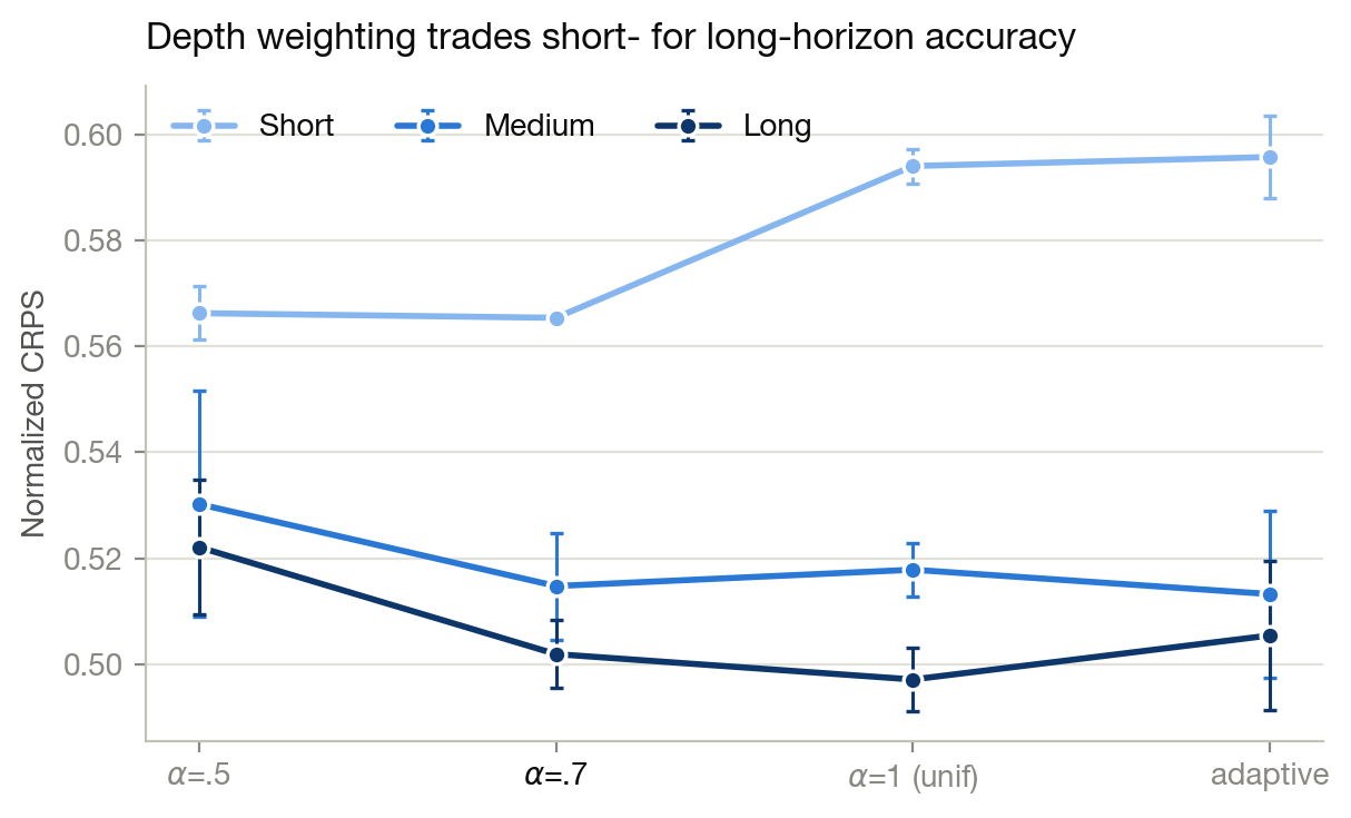
We also tried Dynamic Weight Averaging and three-band GradNorm to try to balance the short and long horizon losses and gradients without luck. Another aspect described above that can probably be simplified after the fix is the recurrence. Recursing only the latent performed well and adding the original embedding and depth seems to improve modestly.
The motivation behind detaching the gradient to the embedding and adding a feedback layer was to alleviate the short-long tradeoff. Deeper losses wouldn’t interfere with the embedding layer that immediate horizons use, while the feedback layer would still let them modify the latents before they entered the transformer. After the data fix, however, detaching embeddings and the feedback layer don’t seem necessary.
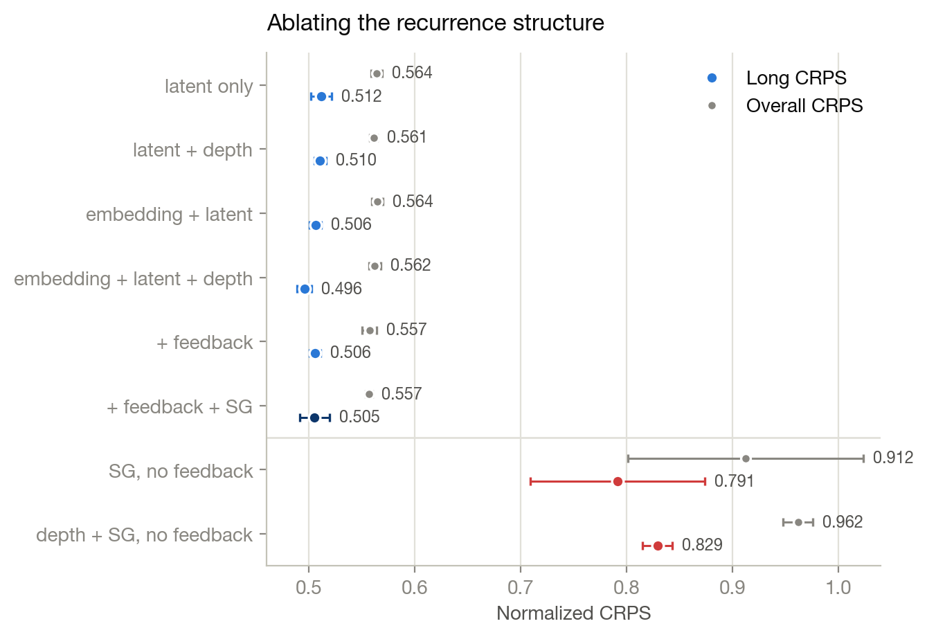
The rollout reach supervised during training turned out to be one of the most important variables. What is surprising, however, is that backpropagating through the recurrence seems unnecessary. A BPTT of 1 still evaluates and supervises all twelve rollout states but stops gradients between adjacent rollouts, suggesting that deep supervision may be sufficient.
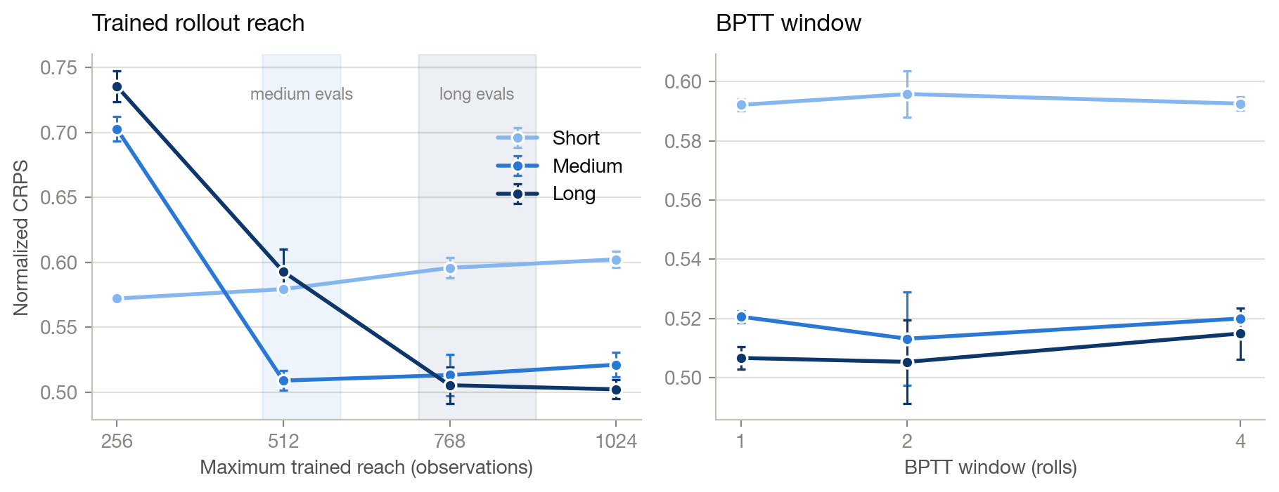
So, as the title of the paper says, it seems that less is indeed more in this forecasting setup and the recursive model should be simpler than those used in the ablations. Adding a latent state and recursing it instead of raw values seems to have at least two advantages. It improves long-horizon distributional forecasts and is conceptually simpler than Moirai’s expand-collapse decoding.
However, training is more expensive 2 and while inference might seem faster because we skip the extra 9 forward passes in the “expand” step, our approach can’t use KV-caching. Moirai can, and can batch extra branching forwards. Thus, actual wall-clock speeds will depend on context length, batching, and implementation.
I’m sure there are lots of ways of pushing this further. For example, randomly truncating rollout depths could speed up training and improving the data pipeline to get greater deep-horizon coverage is sure to help. Making latents stochastic and letting rolls attend or access previous latents beyond the latest one also seem like natural next steps.
We make the code, data, and final simplified checkpoint available and thank Google’s TRC for the compute. Would love comments!