Tiny Recursive Models Pt. 1

a breakdown and some randomization experiments

Published

April 11, 2026

TRMs in a nutshell

A few months ago Hierarchical Reasoning Models (HRMs) showed remarkable ARC performance for their relatively tiny (27M) parameter count. While HRMs introduced a lot of tricks, ablations performed by ARC’s team showed that one (“deep supervision”) accounted for most of the gains. By focusing on “deep supervision”, TRMs greatly simplified and outperformed HRMs with a quarter of the parameters.

TRMs can get away with such small models because they emulate much bigger ones by recursively applying the network on its outputs. They maintain a pair of latent states, \(z\) and \(y\), and refine them until the answer to the input puzzle is predicted by decoding \(y\). Hence we can think of \(y\) as maintaining the embedded answer, which frees up \(z\) to do the “latent reasoning”.

A naive way to train such a model is to backpropagate the loss after all recursions. However, you quickly run out of memory as the model and number of recursions grow. Instead, deep supervision performs a chunk of the recursions (one deep_recursion call in the paper), computes the loss and performs an optimizer step. Then, the latents are detached and used in the next chunk of recursions.

The whole algorithm can be described with 20 lines:

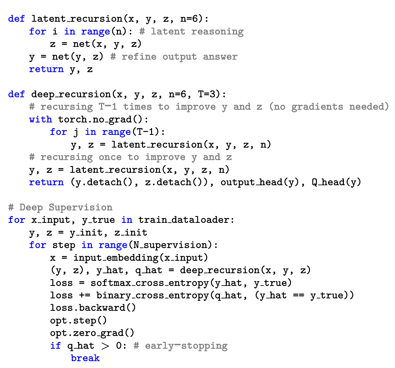
I also made a diagram which omits details but helped me internalize the different recursion levels:

Note that since deep supervision drives most of the performance the algorithm could have been simplified even more by defining:

def deep_recursion(x, y, z, K):
  for i in range(K):
    y, z = net(x, y, z)
  return (y.detach(), z.detach()), output_head(y), Q_head(y)

However, there are a couple of reasons why the paper does not:

Because the network is kept single headed for simplicity, it cannot update \(z\) and \(y\) in a single forward pass.
Related is that latent_recursion allows \(z\) to be updated more frequently than \(y\). We might think that the network is allowed a few “scratchpad” iterations before having to commit to a revised answer. (Note that while intuitive and probably correct, the paper doesn’t perform ablations directly changing the latent’s relative update frequency).
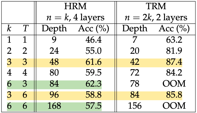
Lastly, the paper recurses a few times (\(T-1\)) without gradients before the final call to latent_recursion with gradients. The argument here is that since deep supervision trains the model to be a “local improver”, it should benefit from running a few extra recursions – even without gradients. However, too many recursions without gradients seem to hurt, as Table 3 shows.

Table 3 from the TRM paper (my highlights)

The last important detail is that deep supervision stops when the network has >50% confidence its predicted solution is correct. This “early-stopping” is turned off during testing for performance but makes training more efficient:

“ACT greatly diminishes the time spent per example (on average spending less than 2 steps on the Sudoku-Extreme dataset rather than the full \(N_\text{sup} = 16\) steps), allowing more coverage of the dataset given a fixed number of training iterations.”

So, that is TRM in a nutshell. The paper does experiments on several tasks (sudokus, mazes, and ARC) and performs lots of ablations (number of latents, architecture, early-stopping, etc.) to show that the choices they landed on are optimal. It also builds up the final design by simplifying HRMs step-by-step and it’s a very pleasant read.

After its publication, others have found simple tweaks that improve performance:

These posts found that simply increasing \(N_\text{sup}\) at test time increases sudoku performance from ~87% to ~96%.
This paper trains the network about 2x faster by using a curriculum on the number of recursions. Instead of the paper’s \((n,T) = (6,3)\), they do \((2,1)\rightarrow(4,2)\rightarrow(6,3)\).
This paper found that if your puzzle admits contractive “milestones” that progressively zero in on the solution, supervising sequentially on those milestones performs better than supervising only on the final solution.

I’m sure there are many more, but those caught my eye. Now, let’s try a few simple experiments!

Experiments

We’ll be using a very simple JAX implementation to use the compute provided by TRC (thank you!) and focus on the sudoku-extreme dataset for now.

Random latent inits for best-of-k at inference

Since increasing the reasoning “depth” (\(N_\text{sup}\)) at test time worked so well, could increasing “breadth” help?

The paper’s implementation initializes \(z\) and \(y\) to random values that are chosen and fixed at model initialization. That is, every forward pass during training and testing starts with the same latents. A simple way to try to get “breadth” is to see if different starting latents are mapped to diverse predictions.

We could then combine or choose among the diverse predictions to make a final one. Normally you would take the majority vote (as test time augmentation (TTA) in vision, or self-consistency in LLMs), but using the model’s own confidence in its prediction (using the halting head) should make more sense here. The paper actually uses both for the TTA they do for ARC, taking the majority vote and breaking ties with model confidence.

Note that it’s not clear that different initializations will get mapped to diverse solutions. It could be that they are ignored because the model maps them to the correct (unique) solution. Or the latents could get numerically “washed away” in the recursion, especially the first \(T-1\) latent recursions without gradient.

We train networks with random latent inits and use the same forward passes to track the performance of predicting the cell-wise majority vote, keeping the whole puzzle the model is most confident in, and just using one of the forward passes as a baseline. Recycling the forward pass makes this the least noisy experiment we’ll make, since training run-to-run variance is really high. However, we also separately train networks with static latent inits as another baseline.

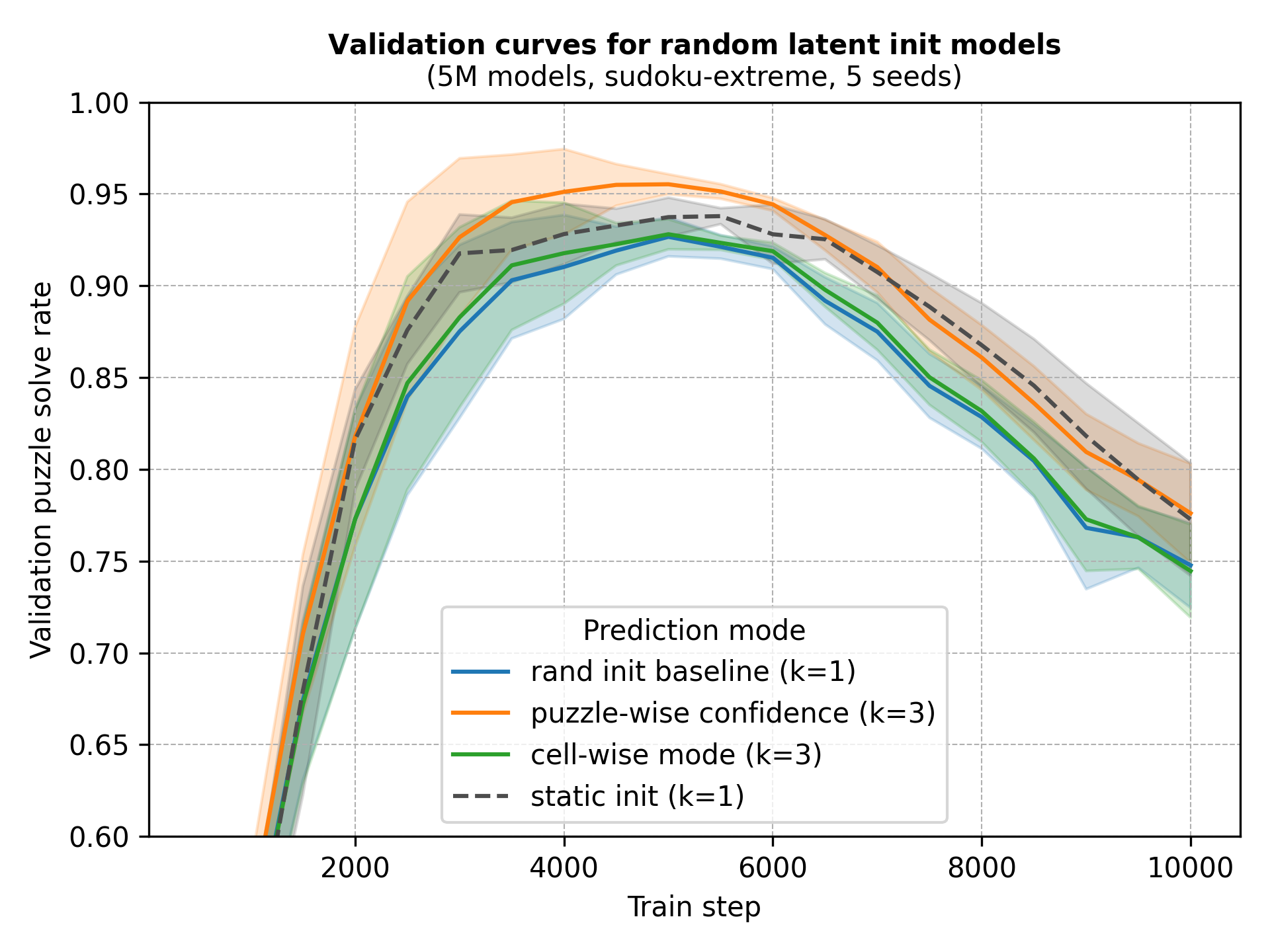
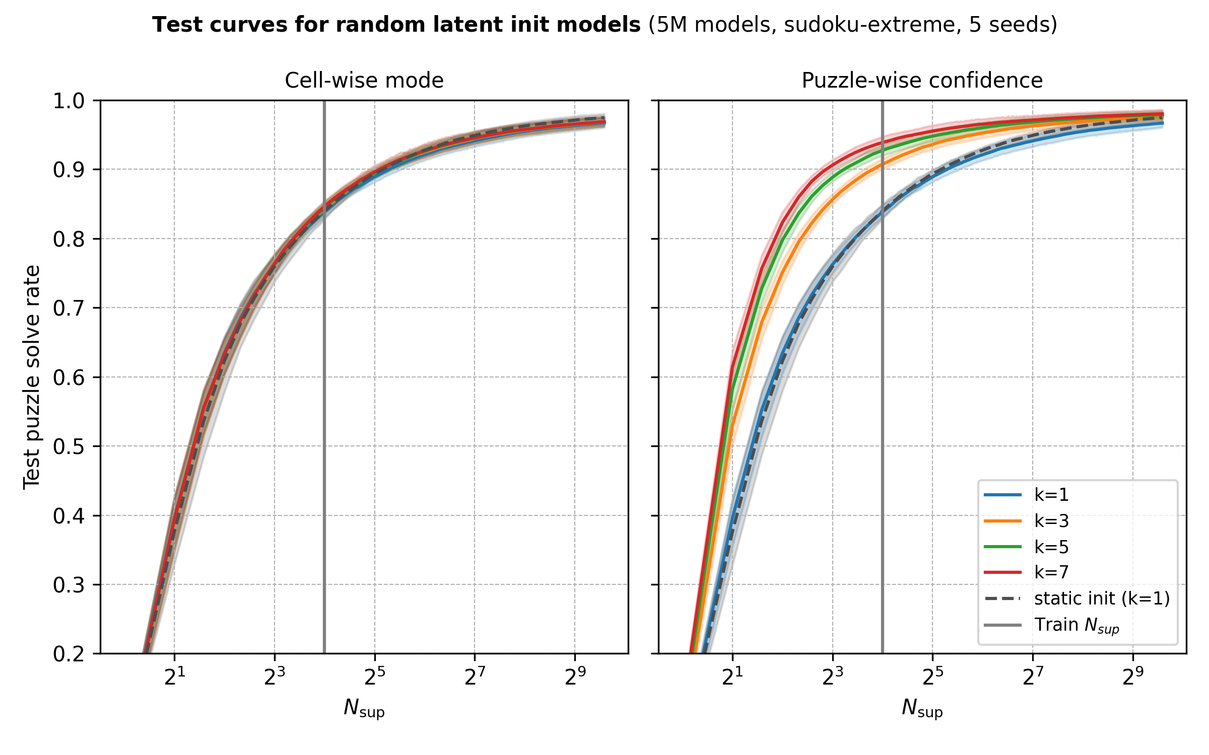
After training we evaluate models with a chunk of the test set using each method’s best validation checkpoint and let \(N_\text{sup}\) and \(k\) grow.

Some observations:

Cell-wise mode seems silly to have tried out in retrospect since cells in sudokus are not independent. As the paper did for ARC, I should have taken puzzle-wise modes. I’ll try to run these at some point.
Random inits paired with model confidence do yield gains and they are most pronounced around (or slightly below) the recursion budget used during training.
As with most test-time scaling methods, increasing \(k\) (and \(N_\text{sup}\)) has diminishing returns.
Methods converge in performance at large recursion budgets.

However, bigger \(k\)’s require more compute and it seems that, at least for this problem and model size, it’s more efficient to scale \(N_\text{sup}\) than \(k\).

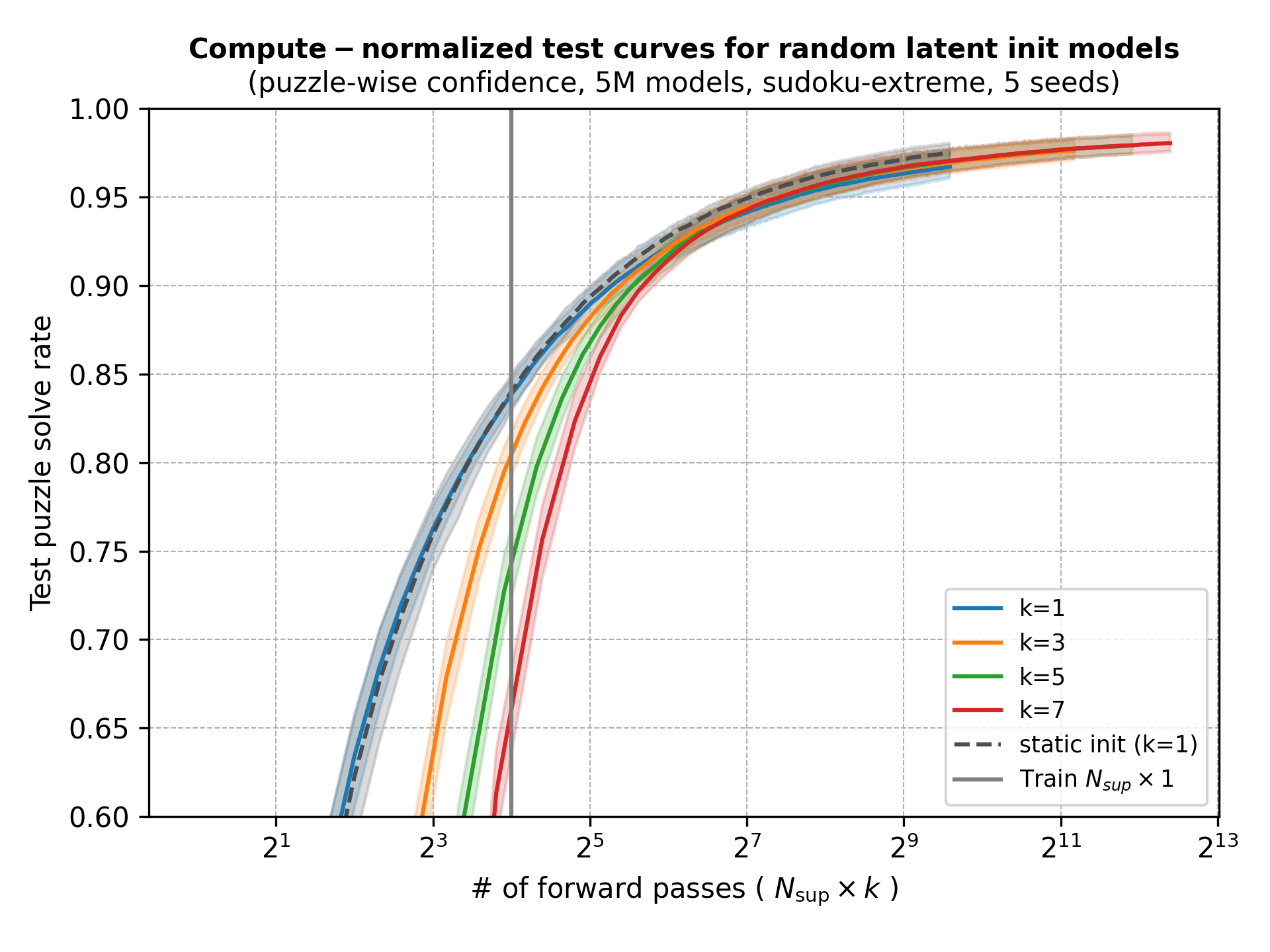
There might be other settings where random initial latents pay off. Maybe problems with multiple solutions or models with underfit predictions but with calibrated halt heads. Anyway, I was mostly surprised that initializations don’t collapse onto the same prediction (at least at low depths) and want to come back to this in the future.

More randomization and path independence

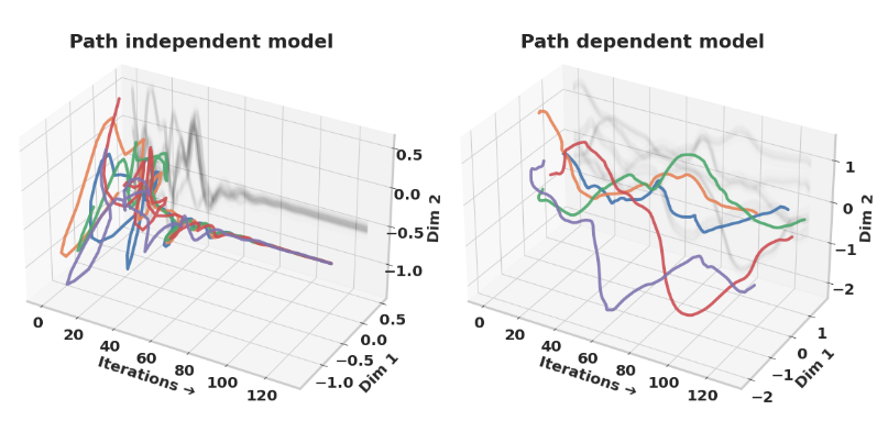
Randomizing initializations do not only allow for test-time augmentation, but have also been shown to stabilize recurrence by helping the model converge to fixed points. Path independent models are those in which latents converge to fixed points regardless of their initial path. The argument is that path independent models are more likely to take advantage of additional iterations by converging to the solution, unlike path dependent models which diverge.

Figure 1 from Path Independent Equilibrium Models Can Better Exploit Test-Time Computation. — Figure 1 from *Path Independent Equilibrium Models Can Better Exploit Test-Time Computation*.

The paper also randomized the number of iterations during training to increase path independence. In our case we could vary \(n\) (the number of iterations in latent_recursion that we spend refining \(z\) before updating \(y\)), \(T\) (the number of “warm-up”, no-gradient latent_recursion calls), and \(N_\text{sup}\) (the number of full \(T(n + 1)\)-sized recursion blocks, and the number of supervision steps).

We could also randomize two or more of these at a time. For example, varying both \(T\) and \(n\) slightly resembles the truncated BPTT with random start and end steps that this paper proposes. However, we keep it simple for now.

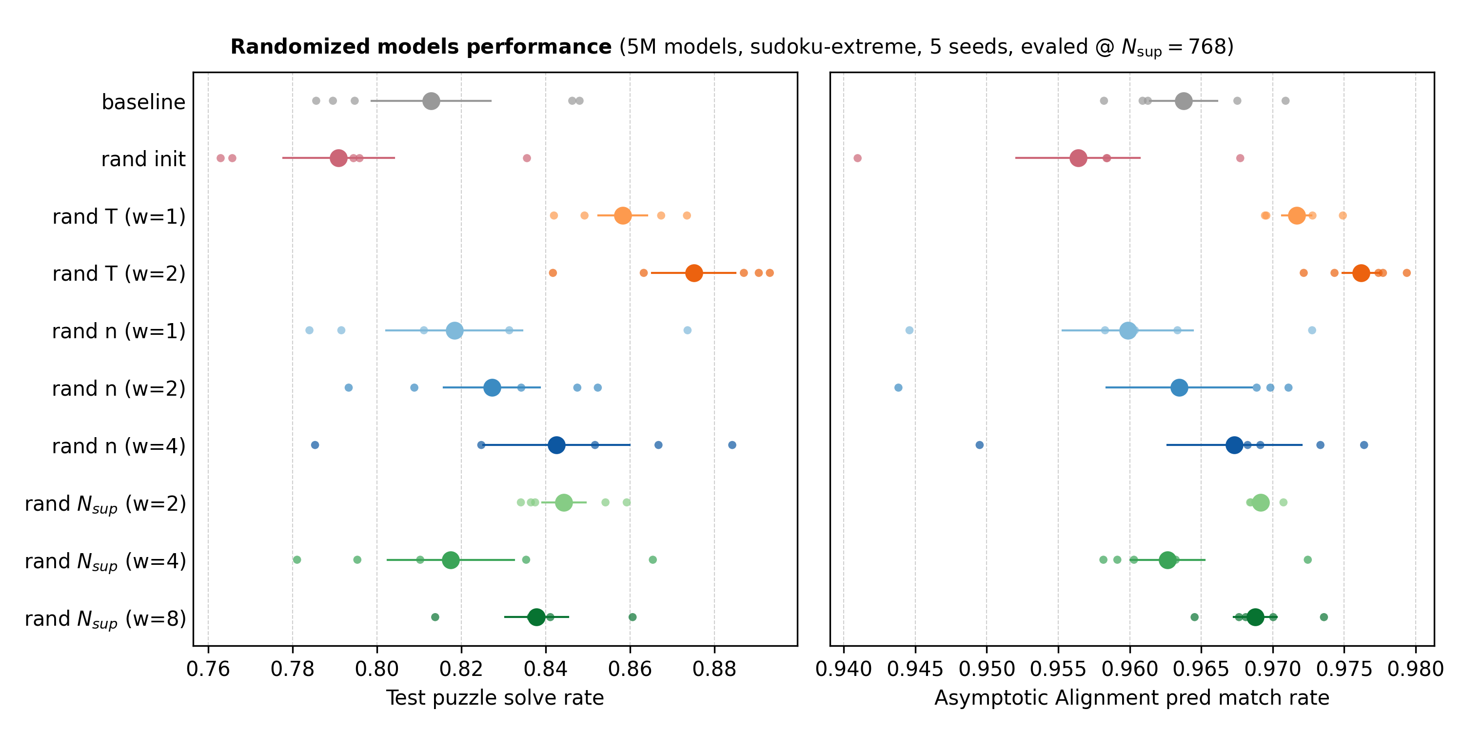
In each training forward pass we sample from uniforms centered at the default values (\(n=6\), \(T=3\), \(N_\text{sup}=16\)) to match the expected compute of deterministic baselines. We try different ranges for these uniforms and keep inference deterministic.

We display mean ± SE and the uniforms’ half-width w. — We display mean ± SE and the uniforms’ half-width \(w\).

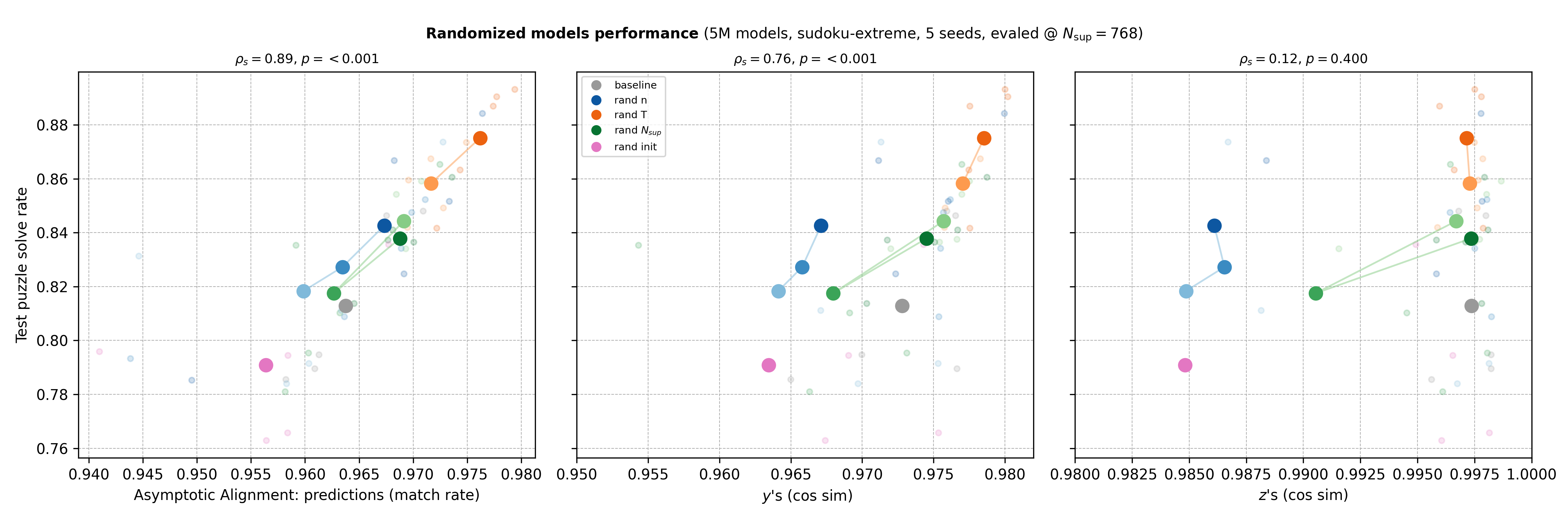
On the right we show the Asymptotic Alignment Score which tries to capture how path independent a network is. It measures the similarity between the final latents of two predictions made for the same data point. The first prediction is initialized normally, but the second uses the first’s final latents. If the similarity is high, the network maps different initializations to the same fixed points and is more path independent. Since we have both latents, we roll both \(z\) and \(y\) for the second forward pass.

Above we plotted the similarity of final predictions instead since we found those to be more consistent. Below we include scores for latents and plot against performance.

Large dots are per-method means; small ones individual seeds. Spearman \rho above each panel. — Large dots are per-method means; small ones individual seeds. Spearman \(\rho\) above each panel.

Even with all the noise from sensitive training and only 5 seeds, we get a few observations:

Like the paper that introduced path independence, we find that it is correlated to performance in this setting.
Reasoning latents (\(z\)’s) saturate and cluster around 1 more so than latent predictions (\(y\)’s). This might be simply because \(z\)’s are updated much more than \(y\)’s.
Surprisingly, random initializations seem to decrease path independence and performance. This doesn’t contradict the path independence paper since their randomization is different. They initialize with zero vectors and only add gaussian noise to half the entries during training, and then use all zeros during testing. I reused the code from previous experiments and randomize during testing too. I’ll try to explore this in a future post.
Even though we increase \(N_\text{sup}\) at test time, it’s randomizing \(T\) during training that yields the biggest gains.
Increasing randomization during training (increasing the uniforms’ range) generally seems to improve performance, with a curious blip in \(N_\text{sup} (w=4)\). To investigate: is the blip real? do gains stack by combining methods? how do gains scale with model capacity?

To be continued

There’s definitely a lot more to learn about and with TRMs. The random initialization idea likely belongs in the paper’s great “Ideas that failed” section and the experiments need polishing. But I thought releasing a first post and iterating would be more fun.